The Law of Diminishing Marginal Productivity is one of the generally accepted economic statements, according to which the application of one new factor of production leads to a decrease in output over time. Most often, this factor is optional, that is, not mandatory in a particular industry. It can be applied intentionally, directly in order to reduce the number of goods produced, or due to a combination of certain circumstances.

What is the theory of diminishing productivity based on?

As a rule, the law of diminishing marginal productivity plays a key role in the theoretical part of production. It is often compared to the waning proposition that occurs in consumer theory. The comparison lies in the fact that the sentence mentioned above tells us how much each individual buyer, and the consumer market in principle, maximizes the produced goods, and also determines the nature of the demand for pricing policy. The law of diminishing marginal productivity affects precisely the steps taken by the manufacturer, the maximization of profits and the dependence of the set price on demand from his side. And in order to make all these complex economic aspects and issues clearer and more transparent for you, we will consider them in more detail and with specific examples.

Pitfalls in the economy

To begin with, let's define the very meaning of the wording of this statement. The law of diminishing marginal productivity is by no means a decrease in the quantity of goods produced in one way or another over the course of all centuries, as it appears on the pages of history textbooks. Its essence lies in the fact that it works only in the case of an invariable, if something is intentionally “inscribed” in the activity that slows down everyone and everything. Of course, this law does not apply in any way when it comes to changing performance features, introducing new technologies, and so on and so forth. In this case, you say, it turns out that the small enterprise has more than its larger counterpart, and this is the essence of the whole question?

Reading the words carefully...

In this case, we are talking about the fact that productivity is reduced due to variable costs (material or labor), which, accordingly, are larger in a large enterprise. The law of diminishing marginal productivity is triggered when this very marginal productivity of a variable factor reaches its maximum in terms of costs. That is why this formulation has nothing to do with increasing the production base in any industry, no matter what it is characterized by. In this matter, we only note that not always an increase in the volume of produced commodity units leads to an improvement in the state of the enterprise and the whole business as a whole. It all depends on the type of activity, because each individual species has its own optimal limit for the growth of production. And if this limit is exceeded, the efficiency of the enterprise, respectively, will begin to decline.

An example of how this complex theory works

So, in order to understand exactly how the law of diminishing marginal productivity works, let's consider it with a clear example. Suppose you are the manager of a certain enterprise. A production base is located on a specially designated area, where all the equipment necessary for the normal functioning of your company is located. And now it's up to you to produce more or less goods. To do this, you need to hire a certain number of workers, draw up an appropriate daily routine, and purchase the right amount of raw materials. The more employees you have, the tighter your schedule, the more foundation you will need for your product. Accordingly, production volumes will increase. It is on this that the law of diminishing marginal productivity of factors that affect the quantity and quality of work is based.

How does this affect the selling price of the product?

We go further and take into consideration the question of Of course, the owner is a gentleman, and he himself has the right to set the desired fee for his goods. However, focusing on market indicators that have long been established by your competitors and predecessors in this field of activity is still worth it. The latter, in turn, tends to constantly change, and sometimes the temptation to sell a certain batch of goods, even if “under-released”, becomes great when the price reaches its maximum on all exchanges. In such cases, in order to sell as many items as possible, one of two options is chosen: increasing the production base, that is, raw materials and the area on which your equipment is located, or hiring more employees, working in several shifts, and so Further. This is where the law of diminishing marginal productivity of returns comes into play, according to which each subsequent unit of the variable factor brings a smaller increment in total production than each previous one.

Features of the decay formula

Many, after reading all this, will think that this theory is nothing but a paradox. In fact, it occupies one of the fundamental positions in economics, and it is based not at all on theoretical calculations, but on empirical ones. The law of diminishing labor productivity is a relative formula derived through many years of observation and analysis of activities in various areas of production. Delving into the history of this term, we note that for the first time it was voiced by a French financial expert named Turgot, who, as a practice of his activity, considered the features of work Agriculture. Thus, for the first time, the "law of diminishing soil fertility" was introduced in the 17th century. He said that a constant increase in the labor applied to a certain plot of land leads to a decrease in the fertility of this plot.

A bit of Turgot's economic theory

Based on the materials that Turgot presented in his observations, the law of diminishing labor productivity can be formulated in the following way: "The assumption that increased costs will give further increased volume of product is always false." Initially, this theory had a purely agricultural background. Economists and analysts argued that on a plot of land, the parameters of which do not exceed 1 hectare, it is impossible to grow more and more crops in order to feed many people with them. Even now, in many textbooks, in order to explain to students the law of diminishing marginal productivity of resources, it is the agricultural industry that is used as a clear and most understandable example.

How it works in agriculture

Let's now try to understand the depth of this issue, which is based on a seemingly banal example. We take a certain plot of land on which more and more centners of wheat can be grown every year. Up to a certain point, each addition of additional seeds will bring an increase in production. But there comes a turning point when the law of diminishing productivity of the variable factor comes into force, which implies that the additional costs of labor, fertilizers and other parts needed in production begin to exceed the former level of income. If you continue to increase production on the same plot of land, then the decrease in former profits will gradually turn into a loss.

But what about the competitive factor?

If we assume that this economic theory has no right to exist in principle, we get next paradox. Let's say growing more and more spikelets of wheat on one plot of land will not be so expensive for the producer. It will be spent on each new unit of its production in the same way as on the previous one, while constantly only increasing the volume of its goods. Consequently, he will be able to perform such actions indefinitely, while the quality of his products will remain the same high, and the owner will not have to purchase new territories for further development. Based on this, we get that the entire amount of wheat produced can be concentrated on a tiny plot of soil. In this case, such an aspect of the economy as competition simply excludes itself.

We form a logical chain

Agree that this theory has no logical basis, since everyone has known since time immemorial that any wheat present on the market differs in price depending on the fertility of the soil on which it was grown. And now we come to the main thing - it is the law of diminishing returns of productivity that is the explanation for the fact that someone cultivates and uses more fertile soil in agriculture, while others are content with soils of lower quality and suitable for such activities. Indeed, otherwise, if every additional centner, kilogram or even gram could be grown on the same fertile plot of land, then no one would have come up with the idea of ​​​​cultivating land less suitable for agricultural industry.

Features of former economic doctrines

It is important to know that in the 19th century, economists still fit this theory exclusively into the field of agriculture, and did not even try to take it out of this framework. All this was explained by the fact that it was in this industry that such a law had the greatest amount of obvious evidence. Among these, one can name a limited production zone (this land plot), rather low rates of all types of work (processing was carried out manually, wheat also grew naturally), in addition, the range of crops that can be grown was quite stable. But given the fact that scientific and technological progress has gradually covered all areas of our lives, this theory quickly spread to all other areas of production.

On the way to modern economic dogmas

In the 20th century, the law of diminishing productivity finally and irrevocably became universal and applicable to all types of activity. The costs that were used to increase the resource base could increase, but without territorial increase, further development simply could not be. The only thing that manufacturers could do without expanding their own boundaries of activity was to purchase more efficient equipment. Everything else - an increase in the number of employees, work shifts, etc. - inevitably led to an increase in production costs, and incomes grew at a much lower percentage compared to the previous indicator.

The law of diminishing productivity plays the same fundamental role in the theory of production as the position of diminishing marginal utility in the theory of consumption. Knowledge of the law of diminishing marginal utility allows us to explain the behavior of a consumer who maximizes total utility and to determine the nature of the demand function of price (demand curve). The law of diminishing productivity underlies the profit-maximizing behavior of the producer and determines the nature and function of supply from price (supply curve).

The law of diminishing productivity does not at all imply a steady decrease in productivity from century to century, this law takes place only under conditions of invariance of any of the factors of production, for example, production technology, the size of the production area. Obviously, in the short run, an increase in output is possible only by attracting additional units of a variable factor of production, while other factors remain constant. Under these conditions, the law of diminishing productivity begins to operate, which states that, starting from a certain moment, each additional unit of the variable factor brings a smaller increment in the total output than the previous one. Thus, the marginal productivity of the variable factor of production sooner or later begins to decline. It is this circumstance that determines the shape of the supply curve: starting from a certain moment, the growth of costs outstrips the growth of output. The manufacturer is forced to offer the product at a higher price. Improvements in technology, for example, or more land, raise the supply curve, increasing productivity. Thus, the law of decreasing productivity (profitability) operates in a short period, and not over a long period of the existence of human society. Let's explain this with an example. Suppose the enterprise has equipment, and workers produce products in one shift. Let's say that the entrepreneur has hired more workers, and the work is now carried out in two shifts. Productivity and profitability are growing. The entrepreneur hires an additional number of workers, organizes work in three shifts. Again, we are seeing an increase in productivity and profitability. But if you continue to hire workers, then there will be no further increase in productivity. Such a constant factor as equipment has already exhausted its possibilities. The application of additional resources to it will no longer have the same effect, on the contrary, starting from this moment, the effectiveness of additional investments will decrease, and the costs per unit of output will increase. If after a few years you change the equipment to a more productive one, then there will be an increase in productivity. For some time, additional investments will lead to increased productivity and profitability. But there will come a time when new, more productive equipment will exhaust itself, and again the effectiveness of additional investments will begin to fall, and the cost of each additional unit will increase.

We see from this example that in order to analyze the operation of an enterprise, only average costs, average profitability and other average values ​​are not enough, but it is necessary to know what these indicators are for each this moment, that is, you need to know the limit values. Thus, the need for marginal analysis in economics is determined by the law of diminishing productivity.

Law of diminishing marginal productivity valid in short term and interval when one factor of production remains unchanged. The operation of the law assumes an unchanged state of technology and production technology, if in manufacturing process the latest inventions and other technical improvements are applied, an increase in output can be achieved using the same production factors. That is, technological progress can change the boundaries of the law.

If a capital is a fixed factor, and work- variable, then the firm can increase production by using more labor resources. But according to the law of diminishing marginal productivity, a consistent increase in a variable resource, while the others remain unchanged, leads to diminishing returns of this factor, that is, to a decrease in the marginal product or marginal productivity of labor. If the hiring of workers continues, then in the end, they will interfere with each other (marginal productivity will become negative) and output will decrease.

Marginal productivity of labor(marginal product of labor - MPL) is the increase in output from each subsequent unit of labor i.e. productivity gain to total product (TPL). The marginal product of capital MPK is defined similarly.

The law of diminishing marginal productivity “states that with an increase in the use of any factor of production (while the others remain unchanged), sooner or later a point is reached at which the additional use of a variable factor leads to a decrease in the relative and further absolute volumes of output. An increase in the use of one of the factors (with the rest fixed) leads to a consistent decrease in the return of its application.

The law of diminishing marginal productivity has never been proven strictly theoretically, it is derived experimentally. If we assume that the law will not be fulfilled, then, for example, it is possible, for example, on a limited plot of land, by increasing the amount of fertilizer, to obtain food for the whole world. This, of course, is not realistic.

The law of diminishing returns begins its operation from the second stage of production, when marginal productivity begins to fall. The level from which the decrease in marginal productivity begins depends on the nature of the production function.

29. The choice of production technology. Isoquant. Marginal rate of technological substitution.

Suppose that only 2 resources are used in production, for example, labor (L) and capital (K) (Figure 5.2). If we connect all combinations of resources, the use of which will provide the same amount of output, then we get isoquants.

An isoquant, or constant product curve, is a curve representing an infinite number of combinations of factors of production that provide the same output.

An isoquant lying above and to the right of another represents a larger volume of output. The set of isoquants, each of which shows the maximum output achieved by using certain combinations of resources, is called an isoquant map.

The marginal rate of technical substitution or technological replacement (MRTS) is the amount of one resource that can be reduced in exchange for a unit of another resource while maintaining the same total output.

The slope of the isoquant measures the marginal rate of technological substitution. The marginal rate of technological substitution shows how much capital can be replaced by one additional unit of labor, provided that output remains unchanged.

30. The rule of cost minimization. Isocost. Producer balance.

The cost minimization rule is as follows: the cost of producing a certain volume of output becomes minimal if the ratio of the marginal product of one factor of production to its price is equal to the ratio of the marginal product of another factor of production to its price: MP 1 /P 1 = MP 2 /P 2, where 1 and 2 are factors of production.

Isocost is a set of points in the plane, each of which corresponds to a set of certain volumes of two factors of production (for example, K - capital and L - labor), acquiring which the entrepreneur will spend the same amount of money.

An isocost map is a graph that shows isocosts corresponding to different levels of an entrepreneur's costs of factors of production.

Using the isocost, it is possible to determine which set of factors of production provides a given output with the lowest total cost (TC). The solution to this problem is at the point of contact (ε) of the isocost with the isoquant, which reflects the equilibrium of the producer.

For a given level of costs, all possible combinations of factors of production must lie on the isocost; at the same time, its slope will reflect the ratio of factor prices (P L /P K). All technologically effective combinations of factors will lie on an isoquant, the slope at each point of which expresses the ratio of marginal factor productivity (MP L /MP K). The optimization condition (MP L /MP K = P L /P K) will be satisfied if the slopes of the isocost and isoquant are equal.

Therefore, the optimum will be reached at the point A of contact between the isoquant and the isocost. For the isoquant, this is the point of replacement of factors of production, expressed in terms of the ratio of their marginal products, for the isocost, the point of replacement of factors of production, expressed in terms of the ratio of their prices.

The minimum production costs are achieved under the condition that the ratio of the marginal productivity of production factors is equal to the ratio of their prices. The condition for minimizing production costs is at the same time the condition under which the equilibrium of the producer is reached, since there is no other combination of factors that can ensure greater production efficiency.

31. Production costs and their classification.

To carry out its activities, the firm incurs certain costs associated with the acquisition of the necessary production factors and the sale of manufactured products. The valuation of these costs is the costs of the firm.

Production costs are the costs of production, expressed in terms of value, associated with the rejection of alternative uses of resources. Production costs - the total cost of living and materialized (past) labor for the production of a product, commodity, service in monetary terms

The principle of alternativeness in determining production costs shows that the actual level of costs should be estimated at the current cost of the resource and taking into account lost profits.

Production costs:

Accounting costs - the actual costs incurred in cash associated with the implementation of production (only payments and accruals that must be taken into account in accordance with legal acts on accounting.)

Economic costs - the opportunity cost of resources diverted from this production. (Explicit, implicit costs)

The costs are:

external ( explicit) - resources purchased by the firm (accounting costs);

Explicit costs- the amount of payments for acquired factors (wages of hired workers, payments to suppliers of material resources, payments on bank loans, payment for transport, energy, etc.).

domestic(implicit, or implicit) - the company's own resources (not reflected in the financial statements).

Implicit costs- this is the cost of services of factors of production that are used in the production process, but are not purchased (for example, belonged to the owner of the firm). Their value is equal to the cash flows that could be obtained under the best alternative use. They are difficult to account for in contracts and are rarely fully valued in cash.

All these costs are usually returnable and are taken into account when making economic decisions along with economic (opportunity) costs.

Return costs are the costs that the firm may not incur by terminating its activities.

Only one category of costs is not taken into account when making important decisions for the firm on the scale of activities - irrevocable. sunk costs associated with previously committed and irrecoverable expenses at the time of closing the company. These include the cost of creating highly specialized equipment, advertising costs, etc.

32. Dynamics of production costs in the short run.

The short run is the period when most of the production remains constant, fixed, and in order to increase (or decrease) the volume of production, the firm can change only one factor of production.

In the long run, the firm can make changes to all factors of production. She can not only hire additional workers but also to build or purchase additional premises and equipment that meet the new market conditions.

In the dynamics of costs in the short term, the following can be distinguished:

• 1. simultaneous reduction of marginal, average variable and total costs;
• 2. decrease in average variables and total averages with an increase in marginal costs;
• 3. increase in marginal and average variables with a decrease in average total costs;
• 4. simultaneous increase in all types of costs.

33. Production costs in the long run.

The long-term production period is the time interval during which the enterprise can change the amount of all employed resources, including the number of production capacities. From an industry point of view, in the long run, there is movement not only within firms to expand or curtail output, but also movement within the industry: some firms leave it, completely curtailing production, and some newly formed ones may come.

In the long run, all factors of production can be changed, and accordingly there will be no division into fixed and variable costs, and only average and marginal costs will be considered. According to its content, long-term production costs reflect changes in costs depending on changes in the scale of production. The nature of these changes will be determined by the type of scale (assuming the prices of factors of production remain unchanged): with a growing scale effect, the average long-term costs will decrease, with a constant one, they will remain unchanged, with a decreasing one, they will increase.

In the long run, the producer can choose any size of production. However, when solving the problem of optimizing production in terms of costs, he must choose such a scale of production at which output would be carried out with the minimum average long-term costs. Under this condition, the optimal size of the enterprise will be such that the equality of long-term average and marginal costs (LMC = LAC) is achieved.

Long run cost curves show the minimum cost of producing any given quantity of output when all factors are variable.

Long-run marginal cost characterizes the increase in costs with an increase in output per unit, if all production resources are variable.

Long-term average costs characterize the specific (average) costs per unit of output, provided that all production resources are variable. The main difference between long-term and short-term analysis is the measure of resource factor elasticity. During long term manufacturers have opportunities that are not feasible in a short period of time. In the long run, the manager can control output and costs by changing not only the intensity production activities per enterprise, but also the size and number of enterprises.

34. Income and profit of the firm.

The cash income that the company receives as a result of the sale of manufactured products takes the form of total (total) income (TR), the value of which depends on the market price (P) of the goods sold and the amount of products sold by the company (Q), i.e. TR = P *Q.

Income can be analyzed both from the standpoint of changes in its total value, and from the standpoint of assessing the profitability of products, as well as the nature of its changes. For this purpose, the indicators of average and marginal income are used. Average income (AR) - the amount of income per unit of product sold, i.e. AR= TR/Q. Marginal income (MR) - the increase in total income from an additional unit of output sold, i.e. MR=ΔTR/ΔQ.

The firm's profit is formed as the difference between total income and total costs, and its changes are described by the function n(q) = TR(q) - TC(q).

Accounting profit is the difference between total revenue and accounting costs, which are actually payments made for the resources involved in the production of goods.

Economic profit is defined as the difference between total revenue and economic costs.

There are two approaches to profit maximization analysis. One of them is based on comparing the absolute values ​​of income and costs, the other is based on marginal analysis and consists in comparing marginal income and marginal costs.

Comparison of total revenue and total costs is based on the fact that the maximum value economic profit will be received when an additionally sold unit of production does not give an increase in profit. The amount of profit is the difference between the total revenue and the total production costs, the values ​​of which functionally depend on the produced and sold quantity of products.

The maximum profit is achieved at the volume q 2 , where the difference between the values ​​of total income and total production costs is the largest (BC). At this level of output, the slope of the total cost curve (point C) is equal to the slope of the total income curve (point B).

The firm maximizes profit at the level of output at which total revenue exceeds total cost of production by the greatest amount.

The comparison of marginal revenue and marginal cost is an example of marginal analysis and relies on the comparison of marginal benefits (MR) and marginal cost (MC) as a maximization principle.

The principle of maximization says that in order to achieve maximum profit, the firm must choose the level of output at which the values ​​of marginal revenue and marginal cost are equal.

35. State regulation of the economy, its forms and methods.

State regulation- a set of measures, actions applied by the state for corrections and the establishment of basic economic processes.

The state is responsible for:

• Fiscal policy (budget, taxes)
• monetary policy ( cash, credit market regulation)
• Regulation of foreign trade
• Regulation of income distribution

Mechanisms of state regulation of market economy:

• Fiscal (fiscal) policy is the activity of the state in the field of taxation, regulation of public spending and the state budget. It is aimed at ensuring the stable development of the economy, preventing inflation and providing employment for the population.
• Monetary (monetary) policy - control over the money supply in the economy. Its goal is to support the stable development of the economy.

Regulation methods are divided into:

• Direct: control over monopolies, ecology, development of standards, their maintenance (quality marks, state standards)
• Indirect: monetary policy, income control, social policy
• Foreign economic regulation

Forms of regulation

• State target programs (social)
• Forecasting
• Situation modeling

State regulation also extends to the technical aspects of activity. This is the so-called "technical regulation". This regulation has common "centralized mechanisms" that are also characteristic of economic regulation: regulation, certification and supervision, licensing, accreditation, delegation, registration, sanctions and appeals.

Reasons for regulation: 1) The presence of public goods in the country (education, health care, environmental protection, etc.) 2) The presence of private and public production 3) The emergence of negative effects within the market (poverty, crime, environmental problems) 4) Scientific and technical progress 5) Tendency towards monopolization 6) Presence of international competition.

36. National economy. National accounting system.

« National economy- this is a system of social reproduction of the country that has historically developed within certain territorial boundaries, an interconnected system of industries and types of production, covering all established forms of social labor.

The ultimate overall goal of the national economy is to provide conditions for the optimal life of all members of society on the basis of economic growth.

This common goal is integrated from a number of more specific goals:

Stable high growth rates of national output

Efficient production

Stability

High level employment, effective employment

Maintenance of foreign trade balance achievement of social justice in the division of society's income.

The basis of the national economy is formed by enterprises, firms, organizations, households, united into a single system by economic relations, performing certain functions in the social division of labor, producing goods and services.

The national economy consists of two major areas: the production of goods (material production) and the provision of services.

System of National Accounts is a balance of interrelated indicators characterizing the production, distribution, redistribution and final use of the final product and national income. At the heart of building a system of national accounting (SNA) is the concept of "economic circulation", the core of which is the economic turnover.

37. Main macroeconomic indicators. Definition of GDP, ways to measure it.

Main macroeconomic indicators:

GDP (gross domestic product) - measures the value of the final product produced in the territory of a given country for a certain period, regardless of whether the factors of production are owned by citizens of this country or owned by foreigners.

GNP (gross national product) - reflects the ownership of the produced product of the nation and differs from GDP by the amount of net factor income from abroad (YF):

GNP=GDP + YF.

Three main methods are used to calculate GDP:

Law of diminishing marginal productivity

The essence of the law.

With an increase in the use of factors, the total volume of production increases. However, if a number of factors are fully involved and only one variable factor increases against their background, then sooner or later there comes a moment when, despite the increase in the variable factor, the total volume of production not only does not grow, but even decreases.

The law says: an increase in a variable factor with fixed values ​​of the rest and the invariance of technology ultimately leads to a decrease in its productivity.

The operation of the law.

The law of diminishing marginal productivity, like other laws, operates in the form of a general trend and manifests itself only when the technology used is unchanged and in a short period of time.

In order to illustrate the operation of the law of diminishing marginal productivity, the following concepts should be introduced:

• - overall product - production of a product with the help of a number of factors, one of which is variable, and the rest are constant;
• - average product - the result of dividing the total product by the value of the variable factor;
• - marginal product - increment of the total product due to the increment of the variable factor per unit.

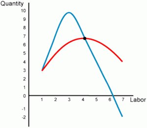
If the variable factor is incremented continuously by infinitesimal values, then its productivity will be expressed in the dynamics of the marginal product, and we will be able to track it on the graph (Fig. 15.1).

Let's build a graph where the main line OAVS - dynamics of the overall product.

• 1. Divide the curve of the total product into several segments: About, VS, SO.
• 2. On the segment OB, we arbitrarily take a point BUT, in which the dynamics of the overall product (OM) coincides with the variable (OR).
• 3. Connect points 0 and BUT - we get D UAR, the angle of which, formed by the sides OA and OR, let's denote a. Attitude AR to OR - middle product, also known as 1§ a.

Rice. 15.1.

4. Draw a tangent to a point BUT. It will intersect the axis of the variable factor at the point N. Formed D APN, where AP/NP- marginal product, also known as tg ß.

On the entire segment Oß tg a< tg ß, т.е. средний продукт меньше предельного. Следовательно, имеется возрастающая отдача от переменного фактора и the law of diminishing marginal productivity does not show its effect.

On the segment Sun the growth of the marginal product is reduced against the background of the continuing growth of the average product. At point C, the marginal and average products are equal to each other and both are equal to tg y. Thus began to appear law of diminishing marginal productivity.

On the segment CD the average and marginal products are reduced, and the marginal product is faster than the average. At the same time, the total product continues to grow. Here the operation of the law is fully manifested.

Behind the dot D, despite the growth of the variable factor, an absolute reduction even of the total product begins. It is difficult to find an entrepreneur who would not feel the effect of the law beyond this point.

Isoquant and isocost. Producer balance. scale effect

Isoquant of output.

The production function can be graphically represented in the form of special curves - isoquants.

Product isoquant - it is a curve showing all combinations of factors within the same output. For this reason, it is often called line of equal output.

Isoquants in production perform the same function as indifference curves in consumption, therefore they are similar: they also have a negative slope on the graph, have a certain proportion of factor substitution, do not intersect with each other, and the farther they are from the origin, the greater the result of production reflect ( Fig. 16.1).

Isoquants can take various forms:

• a) linear - when it is assumed that one factor is completely substitutable for another;
• b) in the shape of an angle when a strict complementarity of resources is assumed, outside of which production is impossible;
• in) broken curve, expressing the limited possibility of replacing resources;
• G) smooth curve - the most general case of the interaction of factors of production (Fig. 16.2).

Marginal rate of technical substitution of resources.

The shift of the isoquant is possible by raising the growth of attracted resources of those

Rice. 16.1.

a, b, c, c1- various combinations; U* U g U g "U) ~ product isoquant

Rice. 16.2.

progress and is often accompanied by a change in its slope. This slope always determines the marginal rate of technical substitution of one factor for another (MRTS). Marginal rate of technical substitution of one factor for another is the amount by which one factor can be reduced by using an additional unit of another factor, while output remains the same:

where L/LG5 is the marginal rate of technical substitution of one factor for another.

Producer balance.

Isoquant - the result of the interaction of factors of production. But in market economy there are no free factors. Consequently, the possibilities of production are not least limited by the financial resources of the entrepreneur. The role of the budget line in this case is played by the isocost.

Isocost - a line that limits the combination of resources to the cash costs of production, so it is often called equal cost line. With its help, the budgetary possibilities of the manufacturer are determined.

The manufacturer's budget constraint can be calculated as follows:

where WITH - manufacturer's budget constraint; r - price of capital services (hourly rent); A "- capital; u> - the price of labor services (hourly wages); I- work.

Even if an entrepreneur does not use borrowed funds, but own funds, this is still a cost of resources, and they should be considered. Factor price ratio g/t shows the slope of the isocost (Fig. 16.3).

Rice. 16.3.

TO- capital; I- work

An increase in the budgetary possibilities of an entrepreneur shifts the isocost to the right, and a decrease to the left. The same effect is achieved in conditions of unchanged costs with a decrease or increase in market prices for resources.

By combining the graphs of isoquant and isocost, one can determine producer balance, those. the optimal set of resources that, with the available financial costs, gives the best result (Fig. 16.4).

The value of the factors used in production is scale of production. Returns to scale (i.e. the result of production activities) can be:

Rice. 16.4.

U r u2 uu ~ isoquants; E- optimum point

• a) permanent, if the result of production increases in the same proportion as resources;
• b) waning, if the result of production increases in a smaller proportion;
• in) increasing if the result of production increases in a larger proportion (Fig. 16.5).

The law reflects the influence of the cost of a variable factor of production on the change in the volume of production, with the constancy of all other factors.

The essence of the law is that if units of a variable resource (labor force) are sequentially added to an invariable factor (equipment), then from a certain moment the marginal product for each subsequent unit of production will not increase, as at the beginning, but decrease.

The law says: an increase in a variable factor with fixed values ​​of the rest and the invariance of technology ultimately leads to a decrease in its productivity.

Let us consider in more detail the operation of the law with an example.

The law of diminishing marginal productivity, like other laws, operates in the form of a general trend and manifests itself only when the technology used is unchanged and in a short period of time.

In order to illustrate the operation of the law of diminishing marginal productivity, one should introduce the concepts:

General product- the production of a product using a number of factors, one of which is variable, and the rest are constant;

Average product- the result of dividing the total product by the value of the variable factor;

marginal product- increment of the total product due to the increment of the variable factor.

If the variable factor is incremented continuously by infinitesimal values, then its productivity will be expressed in the dynamics of the marginal product, and we will be able to trace it on the graph (Figure 6).

Figure 6 - The operation of the law of diminishing marginal productivity

Let's build a graph where the main line OABCB is the dynamics of the total product:

We divide the curve of the total product into several segments: OB, BC, CD.

On the segment OB, we arbitrarily take point A, at which the total product (OM) is equal to the variable factor (OR).

Let's connect the points O and A - we get the RAR, the angle of which from the coordinate point of the graph will be denoted by α. The ratio of AR to OR is the average product, also known as tg α.

Let's draw a tangent to point A. It will cross the axis of the variable factor at point N. APN will be formed, where NP is the marginal product, also known as tg β.

On the entire segment of the OF tg α< tg β, т. е. средний продукт растет медленнее предельного. Следовательно, имеется возрастающая отдача от переменного фактора и закон убывающей предельной производительности своего действия не проявляет.

On segment BC, the growth of marginal product is reduced against the background of the continuing growth of the average product. At point C, marginal product and average product are equal to each other and both are equal to γ. Thus, the law of diminishing marginal productivity began to manifest itself.

On segment CD, the average and marginal products are reduced, and the marginal product is faster than the average. At the same time, the total product continues to grow. Here the operation of the law is fully manifested.

Beyond point D, despite the growth of the variable factor, an absolute reduction even in the total product begins. It is difficult to find an entrepreneur who would not feel the effect of the law beyond this point.

Related information:

1. A) Establishing the conformity of this particular act with the signs of a particular composition of a criminal offense provided for by criminal law.